Cannot collect plots with same fill/color but different geoms

[acircleda]

I'm trying to combine two charts, one using geom_col and one using geom_point. I'd like them to share a legend. They share the same fill/color specification and same colors. I have hidden the legend of one plot, but not the other.

When I use plot_layout(guides = "collect"), it displays one legend, as expected. However, I'd like to add the legend to the top. When I add & theme(legend.position = "top") it then displays both legends, which was not expected.

Here is a simple reprex:

library(palmerpenguins)
library(tidyverse)

penguins %>%
  ggplot(aes(y=species,
             x=body_mass_g,
             fill=sex))+
  geom_col() -> left

penguins %>%
  ggplot(aes(y=species,
             x=body_mass_g,
             color=sex))+
  geom_jitter() +
  theme(legend.position = "none") -> right

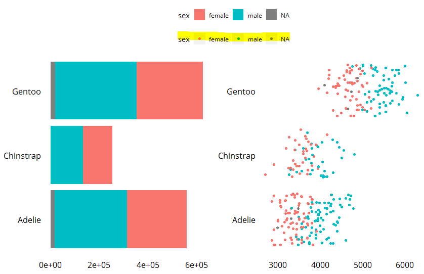
left + right +  plot_layout(guides = "collect") & theme(legend.position = "top")

Here is the output. The highlighted legend should not appear:

[DarwinAwardWinner]

Part of the issue is that you are creating the 2nd legend and then hiding it after the fact. You can get around this problem by never creating the legend in the first place using show.legend = FALSE in the appropriate geom:

library(palmerpenguins)
library(tidyverse)
library(patchwork)

penguins %>%
  ggplot(aes(y=species,
             x=body_mass_g,
             fill=sex))+
  geom_col() -> left

penguins %>%
  ggplot(aes(y=species,
             x=body_mass_g,
             color=sex))+
  geom_jitter(show.legend = FALSE) -> right

left + right +  plot_layout(guides = "collect") & theme(legend.position = "top")

[monkeywithacupcake]

I use the trick that @DarwinAwardWinner uses - suppressing the legend I don't want. However, it is curious that this behavior depends on the class of data being used in the legend.

The penguins$sex variable is a factor. This behavior only happens for characters and factors and not for numeric.

Using the same dataset and example in the current oxygen documentation for plot_layout as a starting point, we can see

#This is the example 
p6 <- ggplot(mtcars) + geom_point(aes(mpg, disp, color=cyl))
p7 <- ggplot(mtcars) + geom_point(aes(mpg, hp, color=cyl))
p6 + p7 + plot_layout(guides='collect')
# results in a plot with ONE GUIDE - as expected

# changing the second plot to a geom_col with a fill aesthetic - like the OP has for the penguin$sex
p6 <- ggplot(mtcars) + geom_point(aes(mpg, disp, color=cyl))
p7fill <- ggplot(mtcars) + geom_col(aes(mpg, hp, fill=cyl))
p6 + p7fill + plot_layout(guides='collect')
# results in a plot with ONE GUIDE 

class(mtcars$cyl) 
#[1] "numeric"

# what if it is another class?

# character
p6 <- ggplot(mtcars) + geom_point(aes(mpg, disp, color=as.character(mtcars$cyl)))
p7fill <- ggplot(mtcars) + geom_col(aes(mpg, hp, fill=as.character(mtcars$cyl)))
p6 + p7fill + plot_layout(guides='collect')
# results in a plot with TWO GUIDES 

# factor
p6 <- ggplot(mtcars) + geom_point(aes(mpg, disp, color=as.factor(mtcars$cyl)))
p7fill <- ggplot(mtcars) + geom_col(aes(mpg, hp, fill=as.factor(mtcars$cyl)))
p6 + p7fill + plot_layout(guides='collect')
# results in a plot with TWO GUIDES

Note that if the second plots, the geom_col() have a color aesthetic - the same aesthetic as the first plot - they still get a second legend, so this is about the treatment of guides of non numeric variables.

[thomasp85]

patchwork relies on exact similarity of the guides to determine if any should be removed. Anything else would open a flood gate of hairy edge cases and surprising behaviour