New tmap v4 defaults
@mtennekes just to keep our discussion in a GitHub issue:
We could consider improving some of the tmap defaults with v4, for example:
- [ ] - color palettes
- [ ] - legends position
- [ ] - legends type (portrait/landscape)
Yes indeed. Ideas and suggestions welcome!
- color palettes: they should at least be color blind friendly
- legends: by default in or outside? Currently I prefer outside, because the device can be used more efficiently. The only case in which inside legends are preferable is when the device has the same aspect ratio as the shape, and when the spatial data is missing in one of the corners (to leave space for a legend)
- legends: by default portrait, landscape, or let it depend on the available space? I'll try to make the last option working: e.g. when a world map of asp ratio of 2:1 is plotted on a 3:1 asp ratio, then a wide landscape legend at the bottom would be the way to go. If on the other hand this world map is plotted on a 1:1 asp ratio device, then a portrait legend is probably better.
- ...
Quick evaluation of the current default color palettes:
# remotes::install_github("nowosad/colorblindcheck")
library(colorblindcheck)
library(RColorBrewer)

# sequential --------------------------------------------------------------
# RdYlGn
YlOrBr = brewer.pal(7, "YlOrBr")
colorblindcheck::palette_check(YlOrBr, plot = TRUE)

#>           name n tolerance ncp ndcp  min_dist mean_dist max_dist
#> 1       normal 7  10.49279  21   21 10.492786  30.41020 61.50052
#> 2 deuteranopia 7  10.49279  21   18  7.764556  26.60910 57.37471
#> 3   protanopia 7  10.49279  21   19  9.015995  30.47439 66.98624
#> 4   tritanopia 7  10.49279  21   19  5.999719  25.22686 54.56822

# diverging ---------------------------------------------------------------
RdYlGn = brewer.pal(7, "RdYlGn")
colorblindcheck::palette_check(RdYlGn, plot = TRUE)

#>           name n tolerance ncp ndcp  min_dist mean_dist max_dist
#> 1       normal 7  8.846536  21   21 8.8465357  35.68053 68.25226
#> 2 deuteranopia 7  8.846536  21   18 0.3022768  22.17456 45.22364
#> 3   protanopia 7  8.846536  21   18 2.0989011  24.73289 58.74541
#> 4   tritanopia 7  8.846536  21   20 6.7951873  33.64488 65.12031

# categorical -------------------------------------------------------------
Set3 = brewer.pal(7, "Set3")
colorblindcheck::palette_check(Set3, plot = TRUE)

#>           name n tolerance ncp ndcp  min_dist mean_dist max_dist
#> 1       normal 7  13.71831  21   21 13.718309  34.40311 55.08545
#> 2 deuteranopia 7  13.71831  21   16  1.971403  25.67463 46.45228
#> 3   protanopia 7  13.71831  21   18  4.754530  25.41755 43.22937
#> 4   tritanopia 7  13.71831  21   19  8.044697  27.76261 55.20569
Created on 2021-09-06 by the reprex package (v2.0.1)
Possible alternatives (any other suggestions are very welcomed!):
# remotes::install_github("nowosad/colorblindcheck")
library(colorblindcheck)

# sequential --------------------------------------------------------------
# RdYlGn
seq = hcl.colors(7, "Red-Yellow")
colorblindcheck::palette_check(seq, plot = TRUE)

#>           name n tolerance ncp ndcp min_dist mean_dist max_dist
#> 1       normal 7  9.164975  21   21 9.164975  32.23835 67.62344
#> 2 deuteranopia 7  9.164975  21   19 6.888086  31.91423 76.87166
#> 3   protanopia 7  9.164975  21   20 7.868990  35.71826 89.92891
#> 4   tritanopia 7  9.164975  21   21 9.583153  27.88259 59.53309

# diverging ---------------------------------------------------------------
div = hcl.colors(7, "Earth")
colorblindcheck::palette_check(div, plot = TRUE)

#>           name n tolerance ncp ndcp  min_dist mean_dist max_dist
#> 1       normal 7  10.97868  21   21 10.978680  26.78995 42.79528
#> 2 deuteranopia 7  10.97868  21   19  9.792442  26.30972 50.01404
#> 3   protanopia 7  10.97868  21   19 10.281933  23.98100 42.55902
#> 4   tritanopia 7  10.97868  21   20 10.629770  30.34651 50.01700

# categorical -------------------------------------------------------------
cat = palette.colors(7, "Okabe-Ito")
colorblindcheck::palette_check(cat, plot = TRUE)

#>           name n tolerance ncp ndcp min_dist mean_dist max_dist
#> 1       normal 7  21.72398  21   21 21.72398  48.10999 88.42242
#> 2 deuteranopia 7  21.72398  21   18 12.99998  44.86723 88.38934
#> 3   protanopia 7  21.72398  21   18 16.17205  42.70554 84.68769
#> 4   tritanopia 7  21.72398  21   16 10.58206  44.38284 80.36656
Created on 2021-09-06 by the reprex package (v2.0.1)
And for bivariate palettes see https://nowosad.github.io/post/cbc-bp2/ and https://nowosad.github.io/colorblindcheck/articles/articles/check_bivariate_pals.html.
My take on this:
* color palettes: they should at least be color blind friendly
I really like this Earth one from above:
* legends: by default in or outside? Currently I prefer outside, because the device can be used more efficiently. The only case in which inside legends are preferable is when the device has the same aspect ratio as the shape, and when the spatial data is missing in one of the corners (to leave space for a legend)
I would tentatively suggest inside to minimise disruption when people upgrade. More examples could be added showing legends outside to get people used using that setting.
* legends: by default portrait, landscape, or let it depend on the available space? I'll try to make the last option working: e.g. when a world map of asp ratio of 2:1 is plotted on a 3:1 asp ratio, then a wide landscape legend at the bottom would be the way to go. If on the other hand this world map is plotted on a 1:1 asp ratio device, then a portrait legend is probably better.
Trust your judgement on that but the current portrait default seems good for many situations. I've had more issues with default legend locations not being great, which I think may be a bigger issue than legend orientation.
Hope that's useful feedback, looking forward to tmap4!
Red-Yellow and Earth are both very nice and harmonic palettes. However, they work better for cases with fewer colors. Hence for picking a general default I would probably go with palettes that give somewhat more discriminability, working for more colors.
In YlOrBr for example you have a slightly larger luminance range and a triangular chroma curve which you do not have in Red-Yellow. Especially the chroma does not only set the extremes (high vs. low) apart but also makes the medium values more distinguishable.
specplot(rev(RColorBrewer::brewer.pal(9, "YlOrBr")), hcl.colors(9, "Red-Yellow"))
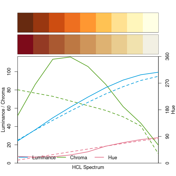
Hence I would probably keep YlOrBr rather than switching to Red-Yellow. Or maybe use YlOrRd which is what image() and filled.contour() are using as the default since R 3.6.0.
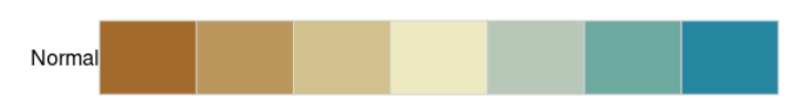
As for Earth: The luminance difference is relatively small (approx 50 in the extremes and 92 in the center). Other palettes go to lower luminances in the extremes (between 20 and 30) which makes them stand out more, e.g., as in BrBG.
specplot(hcl.colors(7, "Earth"), hcl.colors(7, "BrBG"))
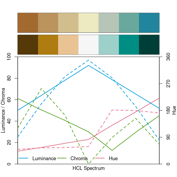
Note that the chroma trajectories in the left and right arm are somewhat unbalanced for both palettes. A more balanced version of BrBG is Green-Brown. Furthermore Purple-Green (and Red-Green) have similar properties.
As for Earth: The luminance difference is relatively small (approx 50 in the extremes and 92 in the center). Other palettes go to lower luminances in the extremes (between 20 and 30) which makes them stand out more, e.g., as in BrBG.
One problem with Earth and BrBG is that they seem to go white or near-white for mid range values. That is a particular problem for maps as you often plot your data on top of a basemap (often black-white) and don't want to lose valuable info. The other suggestions seem to suffer from the 'white centre' issue also, any palettes that do not have this issue, or any other way to mitigate this (I've hit this problem many times)?
library(colorspace)
specplot(hcl.colors(7, "Green-Brown"), hcl.colors(7, "Purple-Green"))

Created on 2021-09-27 by the reprex package (v2.0.1)