Very different plume behavior OBST vs GEOM with and without rotation
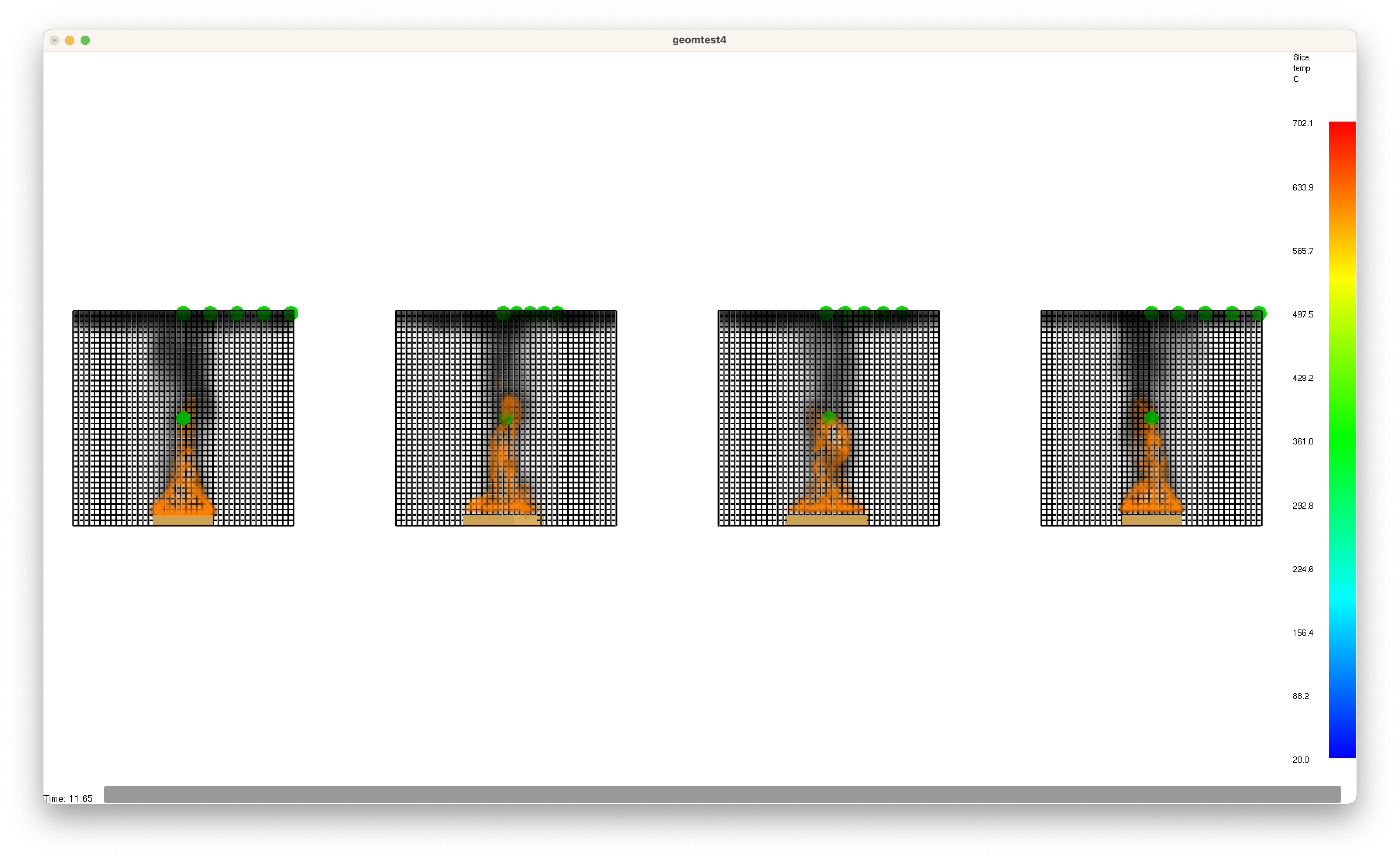
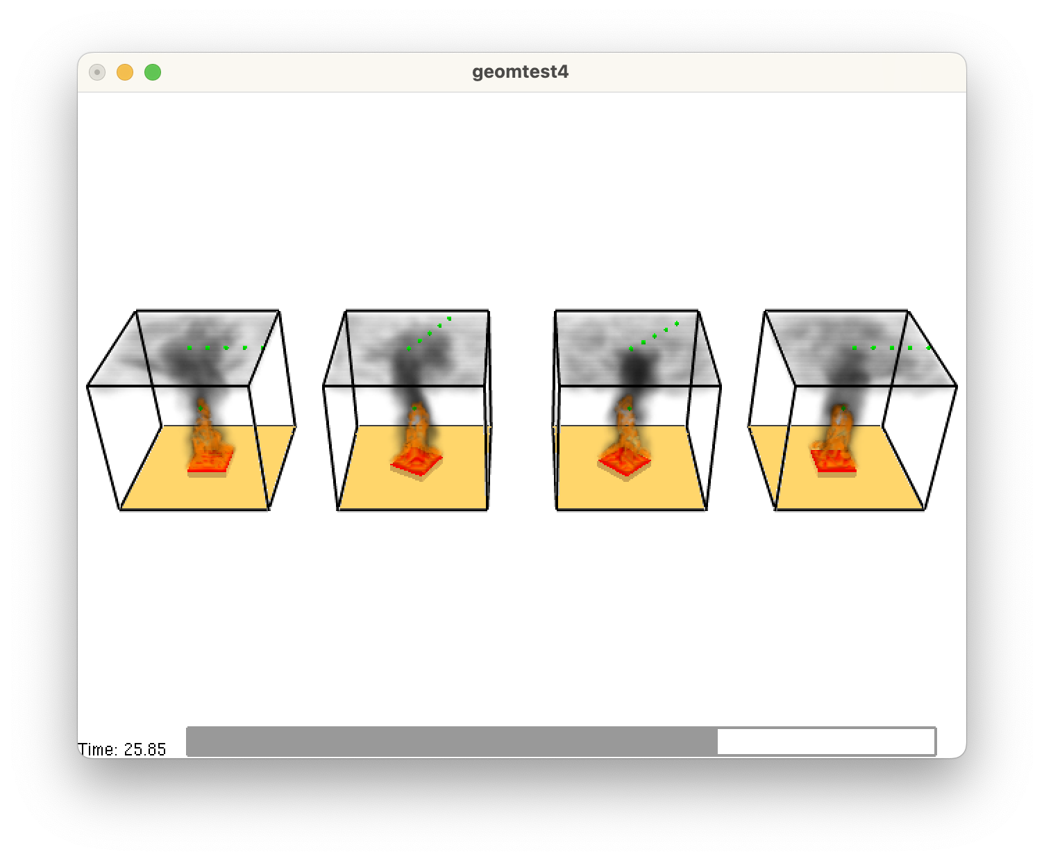
I made a test case with four identical meshes. In each I put a 65 cm x 65 cm burner with
In the first mesh (A) the burner is an OBST In the second (B) the burner is a GEOM and rotated 60 degrees In the second (B) the burner is a GEOM and rotated 45 degrees In the second (D) the burner is a GEOM with no rotation
Each GEOM uses the same XB as the OSBT, just shifted according the MESH XB.
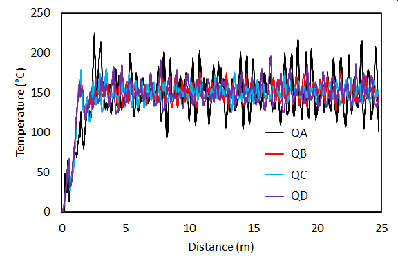
Along the ceiling in each mesh I put a line of TEMPERATURE devices normal to the edge of the burner (i,.e. for mesh A they extend along the x-axis and simply rotate coordinates as needed for the GEOM meshes). I also put devices to integrate the HRRPUV over each mesh
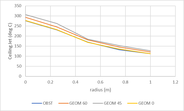
I get very different behavior. The OBST vs. GEOM with no rotation varies considerably and GEOM to GEOM with rotation varies quite a bit as well.
The integrated HRRPUV averaged over 20 s ranges from 150.3 to 151.0 kW. This seems pretty good to me. However, the standard deviation with the OBST is 23 kW and for the three GEOM is 8 to 12 kW. You can clearly in the plot see that the OBST shows much larger swings in the instantaneous HRR.
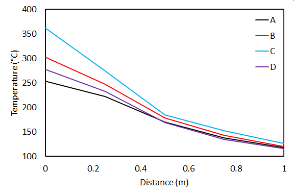
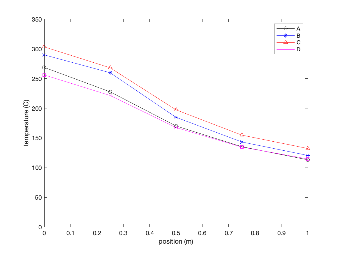
The centerline temperature ranges from 253 C in mesh A to 361 C in mesh C. This is a 50 % difference in temperature rise. Just for the GEOM alone the peak temperatures range from 277 C to 361 C. The GEOM without rotation compared to the equivalent OBST is 253 C for the OBST and 277 C for the GEOM a 10 % difference in temperature rise for what should be geometrically identical cases. The atttached plot shows the temperatures along the ceiling averaged over 20 s.
HRRPUA=500. geomtest4.fds.txt
Thanks, Jason. This is a good test. I suspect the majority of the problem comes from the way the vorticity and stresses are computed near the surface, which affect the local velocity fields, mixing times, etc. I am now starting to turn my attention back to this issue. At the root I think we need to be able to match the Moody chart and ribbed channel flow results first, and we do not yet.
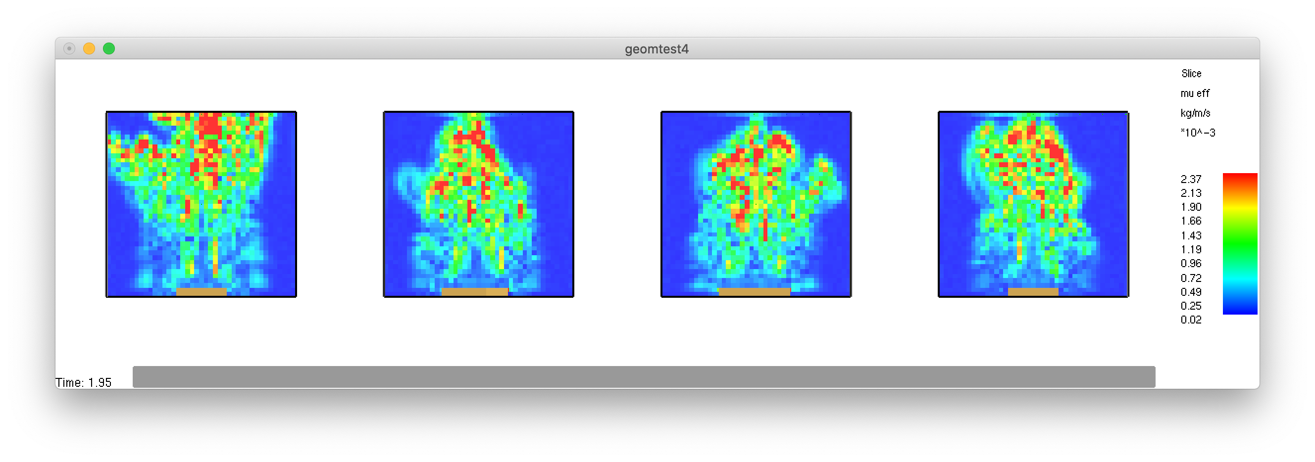
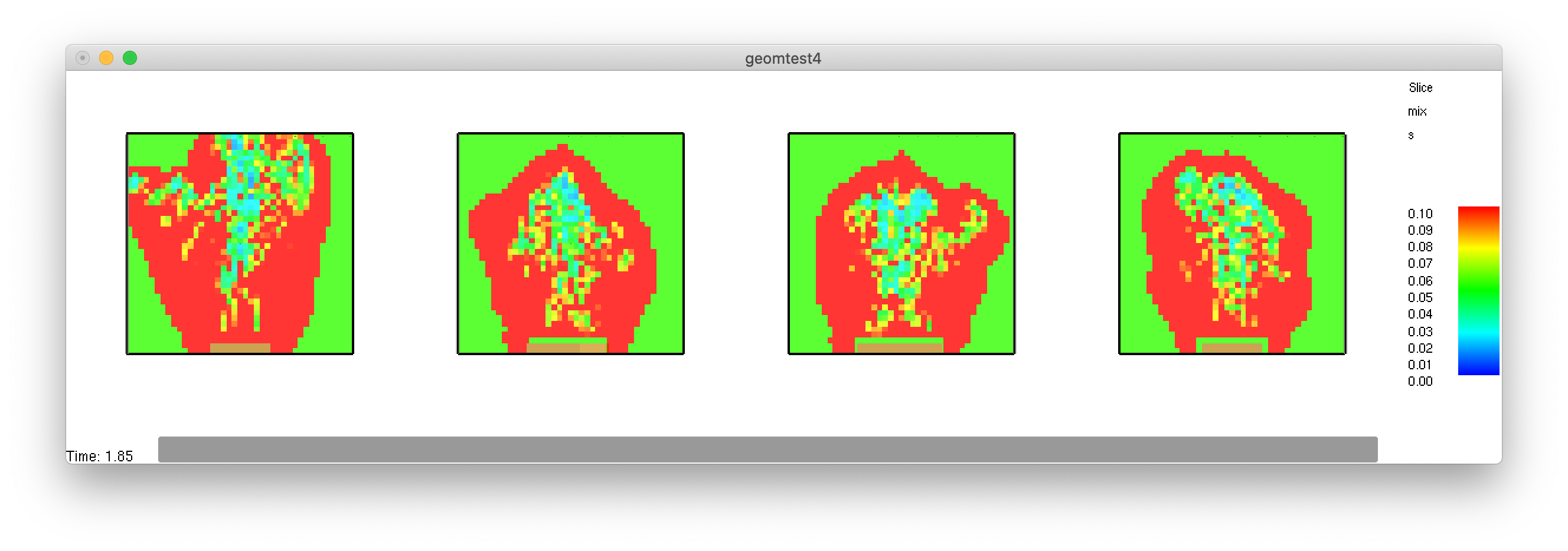
@marcosvanella I'm trying to figure out what is going on with MIX_TIME for CC_IBM. In the images below we see that the VISCOSITY is reasonably consistent, while the MIX_TIME has an obvious jump in the CUT_CELLs. This looks to me to be something other than the wall functions.
Here is VISCOSITY:
And here is the MIX_TIME:
OK, I think the output issue is fixed with PR #8445
I added several output quantities for CC_IBM. But to be strictly correct, any output that derives from ZZ or RHO, etc., need to be put here, and there are many. So, this list will need to grow.
@marcosvanella I noticed here that the initialization for many of the CC_IBM values are simply 0._EB. Please have a look at making these consistent with the values used in init.f90. For example to get MIX_TIME to behave correctly, it needs to be initialized to DT. But this was rough because where you do the init is buried about 5 levels from where DT is available. Perhaps a call to an init routine for CC_IBM needs to be made inside INITIALIZE_MESH_VARIABlES. In that case, feel free to revert the changes I made to argument lists to get MIX_TIME initialized correctly.
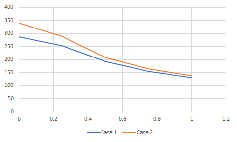
ran this again. Results are much better. Case 1 now matches Case 4 (4 is 1 with GEOM). There is still a noticeable difference in the ceiling jet temperature, though it is less than before especially near the center. Now 6-10 % higher for Case 2 and 9 to 16 % higher for Case 3.
Ran just the first two meshes with a 2x grid refinement. About a 20 % difference at the centerline which decreases to 7 % by the edge.
I need to add the changes that Kevin made to VELOCITY_BC to CC_VELOCITY_BC. Then let's compare again.
With PR #11670 this case qualitatively is looking good. I'll plot the temperatures once it's done.
Jason, this case seems to be slower than I would expect. I guess this is due to UGLMAT. But can you run it through your profiler to see if the pressure solver is indeed the bottleneck here?
I want to make sure I run what you did. Did you add UGLMAT to my input? I didn't specify a solver and geom.f90 sets ULMAT in that case:
! If unstructured projection defined set Pressure solver on unstructured grid.
IF (PRES_FLAG/=UGLMAT_FLAG) THEN
   PRES_METHOD = 'ULMAT'
   PRES_FLAG   = ULMAT_FLAG
ENDIF
Sorry, I think ULMAT is what I meant. I did not change the input file.
Looking at the .out file to confirm... but it looks like we do not say what pressure solver gets used. Is that possible? Holy cow. I'll add that.
The A and D cases are very close. The B and C cases are a bit higher. I think if we wanted to get tighter we'd need to test each case and move the outer boundary farther out. I'm ok with this for now. If you are ok, then close it, else we can keep trying to get closer.
Same basic temp results as before. These results mean that sprinklers will operate quicker if all you do is rotate the burner on the grid. I'll make a case with a t2 fire with a 10 ft ceiling height and see what happens for sprinkler activiation at different distances for different RTI and temperatures. If the fire size at operation winds up close, then I think we can close it.
To be fair, we should also create the rotated cases out of OBST and see what temps we get there.
Started a case on blaze with OBST versions of the two rotations. I kept the same number of OBST cells as the unrotated so the HRRPUA is preserved.
I ran a simulation where I kept the four basic configuratons above plus OBST equivalent of the two rotated GEOM. I made the domain bigger (5 x 5 x 3) and used a t^2 fire. I added fast and standard responses sprinklers with 70, 90, and 110 activation temperatures along the diaganol from the center of the fire to the corner of the domain at 0.5 m increments from the center.
The attached excel sheet has all the results for the various sprinkler operation times and the fire size at that time but a summary is below where O is OBST, G is GEOM, and a number indicates degrees of rotation for the square burner. Values are the average over all sprinklers at that distance and geometry of the fire size at activation divided by the average fire size at that distance for that sprinker. There is a slight tendancy overall for GEOM to have slightly faster times than the grid aligned OBST. The rotated OBST have slower times than GEOM or the grid aligned OBST. I think these results suggest that while there are differences, they are not so large that I consider it a concern. Will close this issue.
| R (m) | O | G=O | G30 | G45 | O45 | O30 |
|---|---|---|---|---|---|---|
| 0 | 0.94 | 0.95 | 0.89 | 0.91 | 1.08 | 1.22 |
| 0.5 | 0.99 | 0.97 | 0.92 | 0.94 | 1.05 | 1.13 |
| 1 | 1.03 | 0.97 | 0.96 | 0.98 | 1.04 | 1.03 |
| 1.5 | 1.03 | 0.97 | 0.96 | 0.99 | 1.03 | 1.01 |
| 2 | 1.04 | 0.97 | 0.98 | 1.00 | 1.03 | 0.99 |
| 2.5 | 1.02 | 0.98 | 0.98 | 1.00 | 1.02 | 1.00 |
| Avg | 1.01 | 0.97 | 0.95 | 0.97 | 1.04 | 1.07 |
geomtest_spk_devc_ctrl_log.xlsx
I like the case. Could we put it on the to-do list for a verification case. I think the rough uncertainty in these nominally equivalent cases is a good thing to publish.