Non constant Young Modulus + arteries disco-elasticity
Hi there,
Thanks for this great library!
It seems that currently configuration files can only take a constant/linear Young's modulus. Do you think adding non-linearity to the modulus would be feasible? Would the solver react properly to this? In addition, arteries have also a viscous component, is this something you are planning to add?
If you believe these additional modelling capabilities would work well with the current solver, I would be happy to help implementing them.
Cheers,
Antoine
Hi Antoine,
that is right, the artery properties are homogeneous along its length with the exception of the lumen radius which can change (linearly). The reason for this is that Young's modulus values are related to the artery radius rather than its length: narrow arteries are stiffer than large ones. In any case, the approach you can use in openBF to model a longitudinal change of E is to split your long artery in several shorter arteries (whit same combined equivalent length) and set a different E for each segment.
In any case, the solver should be able to handle a change in E along z but that has to be first included into the system equations (see appendix A.1 and A.2 from my thesis)
Regarding disco-elastic properties... they're already in the solver! (again, not properly documented sorry)
These are implemented as a parabolic source term right at the end of the solver loop
https://github.com/INSIGNEO/openBF/blob/206854752addd1f75702127ab7ea1cac076a7f2a/src/solver.jl#L227-L241
This system is parameterised on two values WallVa and WallVb which are in turn calculated from a single input parameter phi which you can assign for each artery (by default phi=0.0 and the system is simply elastic)
https://github.com/INSIGNEO/openBF/blob/206854752addd1f75702127ab7ea1cac076a7f2a/src/initialise.jl#L394-L397
This is quite a simple implementation based on the Kelvin-Voigt model but I was able to run the solver fine on few cases. The main problem is to find a fisiological value for phi (eta in the link before) for each artery.
Happy to help more in case you want to share more about your use case
Thanks for your answer, especially for the link to your thesis, it helps understanding the implementation choices!
Regarding the elastic modulus I did not mean a change over the z dimension but rather that the elasticity is not linear. For instance in this plot
 the change in radius is not linear with pressure.
Is this something that could be handled? Or is the solver really relying on the linearity (as it seems from the appendix of your thesis?
the change in radius is not linear with pressure.
Is this something that could be handled? Or is the solver really relying on the linearity (as it seems from the appendix of your thesis?
ah yes, that's a non-linearity that is not taken into account here. The reason is that the physiological range for E is where the curve can be approximated linearly
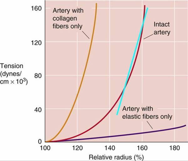
I do not have a reference handy, but you can try to check the relative radius range at the end of one simulation. You'll see that arteries are for most of the time inflated over their nominal size. More importantly, they never collapse as veins do. Collapsing vessels are not really supported by the solver as the collapsing point would create a singularity in the solution. You'd need to switch to a different kind of strategy.
A non-linear E is possible, you'd need to change the constitutive equation
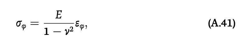 and follow again the derivation in the thesis down to the numerical solver definition.
Depending on your application this could be useful, but I'd say in most of the cases that would be overkill.
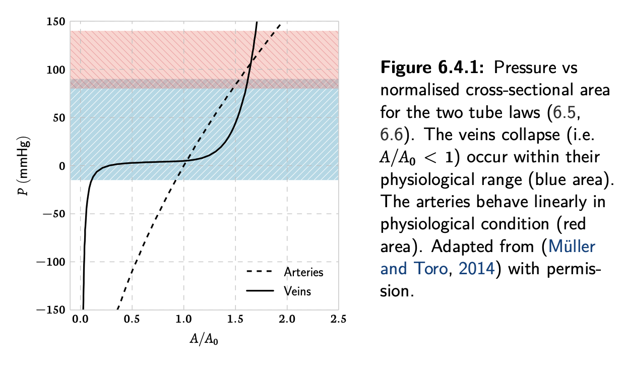
just. found the reference in the thesis, the solver works in the red area. Thus when simulating arteries, the linear assumptions holds
Hi @alemelis!
I am trying to use the viscoelastic parameters phi but I am not able to reproduce some results from the literature although the other effects seem to be well represented by the solver's solutions. By chance, do you have a reference that explain what are WallVa and WallVb and why the lines related to these two parameters correctly handles the effect of phi?
I also wondered whether you had any recommendations on how to chose the parameter gamma_profile? I see in your thesis that you used 2 for "small" arteries and 9 for larger ones but maybe you have some more advice to provide?!
Many thanks in advance.
Cheers,
Antoine
For some context, I am trying to reproduce the results from "Modeling arterial pulse waves in healthy aging: a database for in silico evaluation of hemodynamics and pulse wave indexes". I think more or less all components are not correctly set up except for the viscosity component which I am not managing to get right...
@AWehenkel hello, happy new year!
In order
-
phiis tricky to setup. I do not recall a clear reference on how to use it. Indeed, I eventually dropped it from the thesis and it is not clearly documented in the repository. My understanding at the time was that for a 1D model the effect would be to dampen a bit high frequency oscillation like the ones you may have at a peripheral level. I'll dig into my notes from then and post an update if I find more. -
gamma_profileis discussed in appendix A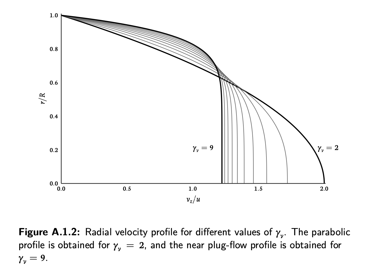 it's a single parameter which lets you shape the velocity profile on the radial direction. It's handy as we have the analytical form of the profile, hence we can integrate along the radius and achieve the 1D system. On the flip side, that equation is a quite coarse approximation of the actual velocity profile. The real one is more like
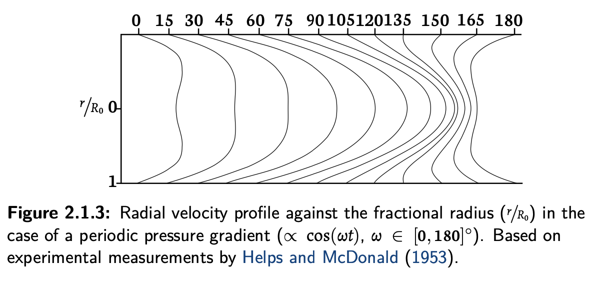 This is time dependent, not constant. On top of that, depending on the vessel radius, viscous forces have a different effect. In general you can assume a larger viscous effect for narrow vessels and set a parabolic profile (gamma=2) while for large arteries (e.g. the aorta) the flow will be plug-like rather than laminar, thus you set gamma=9.
The dream would be to implement a time-dependent Womersley velocity solution and let the solver decide which kind of velocity profile is best at different locations and times. The only study I know with that mechanism in place is [1].
This is time dependent, not constant. On top of that, depending on the vessel radius, viscous forces have a different effect. In general you can assume a larger viscous effect for narrow vessels and set a parabolic profile (gamma=2) while for large arteries (e.g. the aorta) the flow will be plug-like rather than laminar, thus you set gamma=9.
The dream would be to implement a time-dependent Womersley velocity solution and let the solver decide which kind of velocity profile is best at different locations and times. The only study I know with that mechanism in place is [1]. -
regarding that paper...I know of people who allegedly managed to replicate those results but not before fine-tuning all the parameters artery by artery (quite painful process). Anyway, are you trying to match the physiological or numerical results from the paper? Those are very different between each other, I'd be surprised if you couldn't get anything vaguely similar to the physiological ones (at least the pressure ranges and overall waveform shapes).
[1] https://journals.physiology.org/doi/pdf/10.1152/ajpheart.00037.2009
Hi @alemelis,
Happy new year to you as well! Thanks for you your answer.
For gamma it seems [1] sets this parameter to 8/3=2.67 (via a parameter alpha=4/3 and gamma = (2-alpha)/(alpha - 1)) for all vessels from what I have understood of their documentation.
For phi, I have found that [1] uses another parameter called gamma and set it as a function of the diastolic radius as: Gamma(R) = b1/(2100R)+b0/1000 * 1/(piR^2). Gamma is derived from phi: Gamma = 2/3 * sqrt(pi) * phi * h / (piR^2) (as documented in http://haemod.uk/documents/nektar/ReferenceManual.pdf). However trying to use these relationships to derive phi as a function of the diastolic radius: phi(R) = 3/[2 * h(R) * sqrt(pi)] * [b1/(2100R)+b0/1000] does not lead to better results. I think I have correctly checked the units and other things.
I suspect that the problem I have to reproduce the results (numerically) might come from the difficulty I have to take into account tapering with openBF, even when considering non-viscous arteries. Maybe you an idea how to do this properly. I am afraid that openBF assumes that the elasticity is a parameter independent from z whereas [1] defines the "elastic modulus times wall thickness" as a function of the diastolic radius which is a function of z when the arteries are tapered. This aspect could also be a problem for the viscosity. In [1]: Eh(R) = 100 * R * (k1 * np.exp(k2 * 100 * R) + k3)/1000, where k1, k2, k3 are given.
What I have observed is that openBF simulations give decent results when I reproduce [1] and remove tapering (the arteries' radii are made equal to the average between their proximal and distal radii) and then use these radii to set the young modulus from the formula Eh(R) and a formula for h(R). For instance it gives these results:
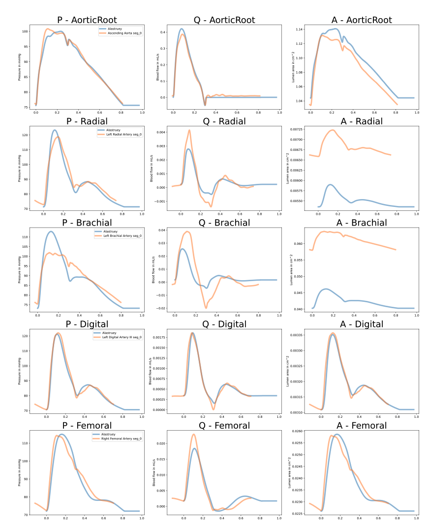 However, we also see that not taking into account the tapering leads to bad waveforms in some arteries (e.g., the brachial in this plot).
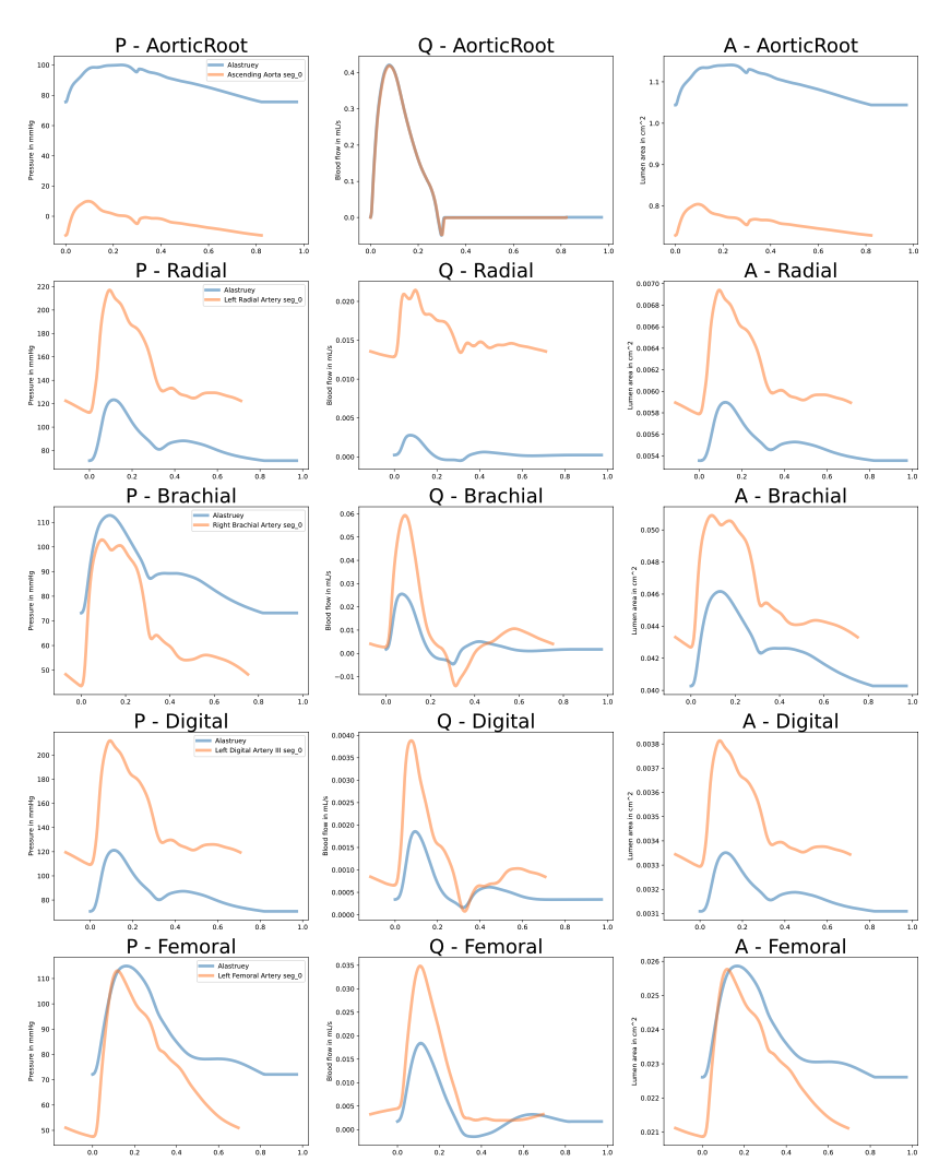
I have tried to simply set the proximal and distal radii to the values given in [1] and the Young's modulus to the same value as above but it leads to very poor results, see the plot below.
However, we also see that not taking into account the tapering leads to bad waveforms in some arteries (e.g., the brachial in this plot).
I have tried to simply set the proximal and distal radii to the values given in [1] and the Young's modulus to the same value as above but it leads to very poor results, see the plot below.
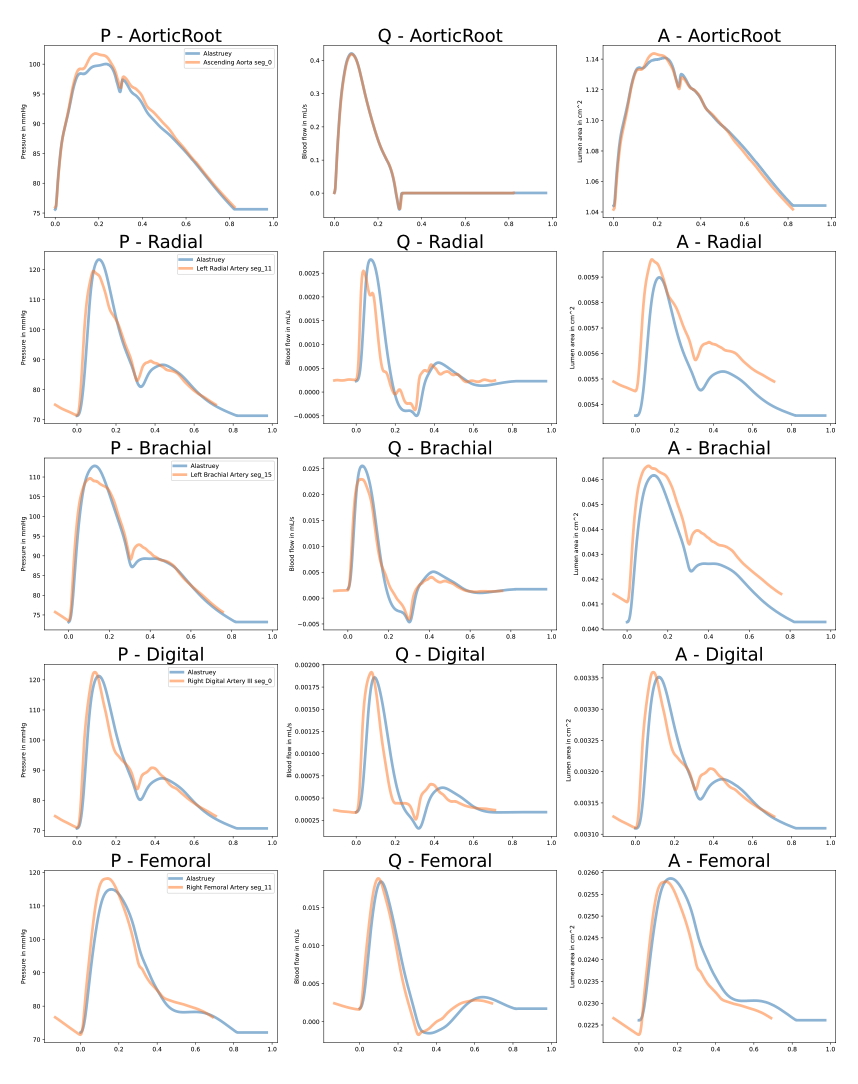
 I have tried to take into account the tapering by splitting the arteries into smaller non-tapered segments (and for each segment the Young's modulus is a function of the radius of the segment) and it gave me what I see as the closest results. However, it also lead to high frequency in some parts, I suppose these are due to reflection appearing on the artificial segments as they have unmatched radii. The results looks like this when I split the vessels into segments of 2centimeters:
So I suppose that the only way to really get something that is closer to [1] would be to properly take into account the tapering of the arteries (and the corresponding effect on their elasticity) but I am not really sure how to do that properly. Or maybe I am simply missing something and not using openBF properly. In any case, I think your help could be very valuable. I know you are not anymore actively doing research on hemodynamics anymore. However, if you are interested, I would be happy to schedule a call and give you more context about the research project I am pursuing.
Sorry for the long answer...
[1]: Charlton, P. H., Mariscal Harana, J., Vennin, S., Li, Y., Chowienczyk, P., & Alastruey, J. (2019). Modeling arterial pulse waves in healthy aging: a database for in silico evaluation of hemodynamics and pulse wave indexes. American Journal of Physiology-Heart and Circulatory Physiology, 317(5), H1062-H1085.
Hi @alemelis,
Sorry for the long absence but I have been quite busy over the last week. I am still planning to add my implementation of heart templates as a function of HR, SV, LVET, ... but at the moment I would really like to find a way of making the tapering work properly. I think I have found potential issues in the current implementation/derivations and I would like to get your opinion about it. I have tried to implement the corresponding changes to the code but I am still obtaining inconsistent results.
I now list the potential issues I have notices:
- In eq 3.1 \alpha, the Coriolis coefficient, is a parameter, this value is then assumed to be equal to 1 in the rest of the derivation. Shouldn't we consider that alpha depends on the fluid/simulation properties? Isn't it related to gamma in some sense?
- Shouldn't source term f_s be multiplied by A (e.g. in eq 3.41 and the following ones)? Indeed we can express dP/dz as the sum of the derivative w.r.t to the different term that depends on z and especially decoupled the dynamic values A from the initial conditions beta_0, A_0. Yet the term A is still a multipliers for the other partial derivatives. It seems this is corrected in the code (https://github.com/INSIGNEO/openBF/blob/206854752addd1f75702127ab7ea1cac076a7f2a/src/solver.jl#L219).
- The line https://github.com/INSIGNEO/openBF/blob/206854752addd1f75702127ab7ea1cac076a7f2a/src/solver.jl#L219 seems to miss the term relative to dP/dA_0 and I think the way you compute dtau/dx misses to account for the partial derivative of A_0 w.r.t to z. I have made the corresponding modifications to this source term by accounting for all changes in P for a change in z and indeed obtain a different source term than yours. However I still obtain weird curves that goes into negative pressure while taking the two corresponding simulations without any tapering, respectively with R0=Rp and R0=Rd the curves are positive. I would expect the corresponding tapered curves to be somehow an interpolation between these two cases, at least I do not see why tapering would suddenly provide negative pressures.
- It seems the implemented superbee is not similar as the one described in the thesis, do you know why is it so?
- I wonder if the rate of tapering/change in Eh0 as z changes could also impact the wave speed somehow and so the Riemann invariants and interface conditions?!
- I do not understand how you obtain the Jacobian in 3.42. Why isn't H_11 equal to u? and why is H21=3/2gamma x sqrt(A)-u^2 shouldn't it be H21=3/2gamma x sqrt(A) + u^2... What am I missing?
Sorry again for the long message, hopefully we might find a way to get the tapering correct! :D
Cheers,
Antoine
hello @AWehenkel !
I'll try to answer to these one by one...
- true, alpha should change when changing gamma (they are related). In order to simplify the equations, it is assumed always
alpha=1and we approximategamma → ∞asgamma=9. This is a limitation of using a fixed velocity profile instead of simulating one. Again, the solver is mainly focused on simulating blood flow in large elastic arteries, wheregamma=9is fine. The option to setgamma=2for smaller vessels is with the aim of recovering (numerically) some of the viscous losses without changing the equations (which you should do withalpha != 1). In any case,alpha=1simplifies a lot the calculation of characteristics (resulting inu ± c) and it is a standard practice in the field. In physiological cases,alpha>1and the characteristics should beu ± sqrt(alpha*(alpha - 1)*u^2 + c^2); you can see how this will make the next steps more difficult to handle. - need to check, this is the reason why I started the
v2branch. I'm far from being at that point of the analysis. Happy to have some help here in refactoring the source terms to an intelligible form. - as for 2
- you are right, seems like the average term is missing. That probably needs to be fixed! The superb function is to limit slopes and avoid the solver to explode. (thinking out loud) Without that average factor the slopes are allowed to be larger than expected, thus this could explain segfaulting simulations. However, converging cases shouldn't get different results. Good catch! 🎣
- The wave speed (hence the RI) is definitely linked to
E*h0, but that is not supposed to change dramatically within an artery even when tapering occurs (talking about phisiological cases). When you have a section where you know that a big change inEorh0occurs, you should split the vessel in two segments and let the solver deal with the discontinuous interface rather than having discontinuities in the parameters. - ehe, that's the most confusing part of the process in my opinion. I remember I spent quite a long time to check that derivation, and most likely I was following the steps from [1] which I could borrow from the university library. The same Jacobian is reported in [2] but the derivation is not provided.
[1] Modeling of Physiological Flows (2011) google books page [2] Well-balanced high-order numerical schemes for one-dimensional blood flow in vessels with varying mechanical properties journal link